
4. Affordable and Clean Energy
Affordable and Clean Energy is the 7th Sustainable Development Goal 11. It aspires to ensure access to affordable, reliable, sustainable and modern energy for all. Today renewable energy is making impressive gains in the electricity sector. As more and more new settlements are built, there would be new electricity distribution network developed. Electricity Distribution is very expensive infrastructure. Finding the optimal path for laying this infrastructure is very crucial to maintain the affordability of electricity for everyone. This exercise focusses on finding this optimal path/network for laying the electricity distribution equipment.

4.1. Problem: Optimising the Electricity Distribution Network
Problem Statement
To determine the least length of the path for laying the electricity distribution equipment such that every building is served
Core Idea
Electricity lines may not be there on every road of the city. In a complex road network of a city, the network can be optimised for less length such that Electricity lines reach every locality of the city. Less length leads to enhanced cost-effectiveness resulting in affordable electricity.
Approach
Extract connected components of roads
Use pgRouting to find the minimum spanning tree
Compare the total length of roads and minimum spanning tree
4.2. Pre-processing roads data
First step is to pre-process the data obtained from Data for Sustainable Development Goals. This section will work the graph that is going to be used for processing. While building the graph, the data has to be inspected to determine if there is any invalid data. This is a very important step to make sure that the data is of required quality. pgRouting can also be used to do some Data Adjustments. This will be discussed in further sections.
4.2.1. Setting the Search Path of Roads
First step in pre processing is to set the search path for Roads data.
Search path is a list of schemas helps the system determine how a particular table
is to be imported.
4.2.1.1. Exercise 1: Inspecting the current schemas
Inspect the schemas by displaying all the present schemas using the following command
\dn
   List of schemas
   Name    |  Owner
-----------+----------
 public    | postgres
 roads     | <user-name>
(2 rows)
The schema names are roads and public. The owner depends on who has the rights to the database.
4.2.1.2. Exercise 2: Inspecting the current search path
Display the current search path using the following query.
SHOW search_path;
   search_path
-----------------
 "$user", public
(1 row)
This is the current search path. Tables cannot be accessed using this.
4.2.1.3. Exercise 3: Fixing the current search path
In this case, search path of roads table is set to roads schema. Following query
is used to fix the search path
SET search_path TO roads,public;
SHOW search_path;
    search_path
-------------------
 roads, public
(1 row)
4.2.2. Exercise 4: Enumerating the tables
Finally, \dt is used to verify if the Schema have bees changed correctly.
\dt
                     List of relations
  Schema   |            Name             | Type  |  Owner
-----------+-----------------------------+-------+---------
 public    | spatial_ref_sys             | table | <user-name>
 roads     | configuration               | table | user
 roads     | roads_pointsofinterest      | table | user
 roads     | roads_ways                  | table | user
 roads     | roads_ways_vertices_pgr     | table | user
(5 rows)
4.2.3. Exercise 5: Counting the number of Roads
The importance of counting the information on this workshop is to make sure that the same data is used and consequently the results are same. Also, some of the rows can be seen to understand the structure of the table and how the data is stored in it.
1-- Counting the number of Edges of roads
2SELECT count(*) FROM roads_ways;
3
4-- Counting the number of Vertices of roads
5SELECT count(*) FROM roads_ways_vertices_pgr;
4.3. pgr_connectedComponents for preprocessing roads
For the next step pgr_connectedComponents will be used. It is used to find the
connected components of an undirected graph using a Depth First Search-based approach.
Signatures
pgr_connectedComponents(edges_sql)

RETURNS SET OF (seq, component, node)
OR EMPTY SET
pgr_connectedComponents Documentation can be found at this link for more information.
4.4. Extract connected components of roads
Similar to Good Health and Well Being, the disconnected roads have to be removed from their network to get appropriate results.
Follow the steps given below to complete this task.
4.4.1. Exercise 6: Find the Component ID for Road vertices
First step in Preprocessing Roads is to find the connected component ID for Road vertices. Follow the steps given below to complete this task.
Add a column named
componentto store component number.
1ALTER TABLE roads_ways_vertices_pgr
2ADD COLUMN component INTEGER;
Update the
componentcolumn inroads_ways_vertices_pgrith the component number
1UPDATE roads_ways_vertices_pgr
2SET component = subquery.component
3FROM (
4	SELECT * FROM pgr_connectedComponents(
5		'SELECT gid AS id, source, target, cost, reverse_cost
6		FROM roads_ways')
7		)
8AS subquery
9WHERE id = node;
This will store the component number of each edge in the table. Now, the completely
connected network of roads should have the maximum count in the component table.
if done before: Exercise: 10 (Chapter: SDG 3) if not done before: Exercise: 6 (Chapter: SDG 7)
4.4.2. Exercise 7: Finding the components which are to be removed
This query selects all the components which are not equal to the component number
with maximum count using a subquery which groups the rows in roads_ways_vertices_pgr
by the component.
 1WITH
 2subquery AS (
 3	SELECT component, count(*)
 4	FROM roads_ways_vertices_pgr
 5	GROUP BY component
 6	)
 7SELECT component FROM subquery
 8WHERE count != (
 9	SELECT max(count) FROM subquery
10);
if done before: Exercise: 11 (Chapter: SDG 3) if not done before: Exercise: 7 (Chapter: SDG 7)
4.4.3. Exercise 8: Finding the road vertices of these components
Find the road vertices if these components which belong to those components which are to be removed. The following query selects all the road vertices which have the component number from Exercise 7.
 1WITH
 2subquery AS (
 3	SELECT component, count(*)
 4	FROM roads_ways_vertices_pgr
 5	GROUP BY component),
 6	to_remove AS (
 7		SELECT component FROM subquery
 8		WHERE count != (
 9		SELECT max(count) FROM subquery
10	)
11)
12SELECT id FROM roads_ways_vertices_pgr
13WHERE component IN (SELECT * FROM to_remove);
if done before: Exercise: 12 (Chapter: SDG 3) if not done before: Exercise: 8 (Chapter: SDG 7)
4.4.4. Exercise 9: Removing the unwanted edges and vertices
Removing the unwanted edges
In roads_ways table (edge table) source and target have the id of
the vertices from where the edge starts and ends. To delete all the disconnected
edges the following query takes the output from the query of Step 4 and deletes
all the edges having the same source as the id.
 1DELETE FROM roads_ways WHERE source IN (
 2		WITH
 3		subquery AS (
 4			SELECT component, count(*)
 5			FROM roads_ways_vertices_pgr
 6			GROUP BY component
 7			),
 8		to_remove AS (
 9			SELECT component FROM subquery
10			WHERE count != (
11				SELECT max(count) FROM subquery
12				)
13	)
14	SELECT id FROM roads_ways_vertices_pgr
15	WHERE component IN (SELECT * FROM to_remove)
16);
Removing unused vertices
The following query uses the output of Step 4 to remove the vertices of the disconnected edges.
 1WITH
 2subquery AS (
 3	SELECT component, count(*)
 4	FROM roads_ways_vertices_pgr
 5	GROUP BY component
 6	),
 7	to_remove AS (
 8		SELECT component FROM subquery
 9		WHERE count != (SELECT max(count) FROM subquery)
10		)
11	DELETE FROM roads_ways_vertices_pgr
12	WHERE component IN (SELECT * FROM to_remove
13);
if done before: Exercise: 13 (Chapter: SDG 3) if not done before: Exercise: 9 (Chapter: SDG 7)
4.5. pgr_kruskalDFS
For the next step pgr_kruskalDFS will be used. Kruskal algorithm is used for
getting the Minimum Spanning Tree with Depth First Search ordering. A minimum spanning
tree (MST) is a subset of edges of a connected undirected graph that connects all
the vertices together, without any cycles such that sum of edge weights is as small
as possible.
Signatures
pgr_kruskalDFS(Edges SQL, Root vid [, max_depth])
pgr_kruskalDFS(Edges SQL, Root vids [, max_depth])

RETURNS SET OF (seq, depth, start_vid, node, edge, cost, agg_cost)
Single vertex
pgr_kruskalDFS(Edges SQL, Root vid [, max_depth])

RETURNS SET OF (seq, depth, start_vid, node, edge, cost, agg_cost)
Multiple vertices
pgr_kruskalDFS(Edges SQL, Root vids [, max_depth])

RETURNS SET OF (seq, depth, start_vid, node, edge, cost, agg_cost)
pgr_kruskalDFS Documentation can be found at this link for more information.
4.6. Exercise 10: Find the minimum spanning tree
The road network has a minimum spanning forest which is a union of the minimum spanning trees for its connected components. This minimum spanning forest is the optimal network of electricity distribution components.
To complete this task, execute the query below.
1SELECT source,target,edge, r.the_geom
2FROM pgr_kruskalDFS(
3    'SELECT gid AS id, source, target, cost, reverse_cost, the_geom
4    FROM roads.roads_ways ORDER BY id',
5    91),
6roads.roads_ways AS r
7WHERE edge = r.gid
8LIMIT 10;
The following query will give the results with the source vertex, target vertex, edge id, aggregate cost.
1SELECT source,target,edge,agg_cost
2FROM pgr_kruskalDFS(
3    'SELECT gid AS id, source, target, cost, reverse_cost, the_geom
4    FROM roads.roads_ways
5    ORDER BY id',91),
6roads.roads_ways AS r
7WHERE edge = r.gid
8ORDER BY agg_cost
9LIMIT 10;
Note
LIMIT 10 displays the first 10 rows of the output.
4.7. Comparison between Total and Optimal lengths
Total lengths of the network and the minimum spanning tree can be compared to see the difference between both. To do the same, follow the steps below:
4.7.1. Exercise 11: Compute total length of material required in km
Compute the total length of the minimum spanning tree which is an estimate of the total length of material required.
 1SELECT SUM(length_m)/1000
 2FROM (
 3	SELECT source,target,edge,agg_cost,r.length_m
 4	FROM pgr_kruskalDFS(
 5		'SELECT gid AS id, source, target, cost, reverse_cost, the_geom
 6		FROM roads.roads_ways
 7		ORDER BY id',91),
 8	roads.roads_ways AS r
 9	WHERE edge = r.gid
10	ORDER BY agg_cost)
11AS subquery;
Note
(length_m)/1000 is used to fine the length in kilometres
4.7.2. Exercise 12: Compute total length of roads
Compute the total length of the road network of the given area..
1SELECT SUM(length_m)/1000 FROM roads_ways;
Note
(length_m)/1000 is used to fine the length in kilometres
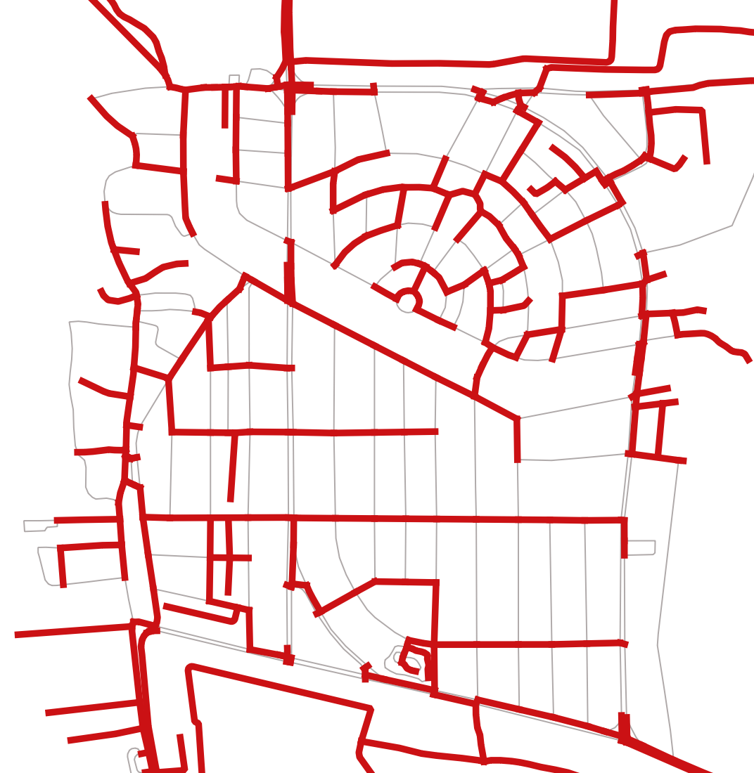
For this area we are getting following outputs:
Total Road Length:
55.68 kmOptimal Network Length:
29.89 km
Length of minimum spanning tree is about half of the length of total road network.
4.8. Further possible extensions to the exercise
Finding the optimal network of roads such that it reaches every building
Finding the optimal number and locations of Electricity Transformers