3. Good Health and Well Being ¶

Good Health and Well Being is the 3rd Sustainable Development Goal which aspires to ensure health and well-being for all, including a bold commitment to end the epidemics like AIDS, tuberculosis, malaria and other communicable diseases by 2030. It also aims to achieve universal health coverage, and provide access to safe and effective medicines and vaccines for all. Supporting research and development for vaccines is an essential part of this process as well as expanding access to affordable medicines. Hospitals are a very important part of a well functioning health infrastructure. An appropriate planning is required for optimal distribution of the population of an area to its hospitals. Hence, it is very important to estimate the number of dependant people living near the hospital for better planning which would ultimately help in achieving universal coverage of health services. This chapter will focus on solving one such problem.

Image Source

3.1. Problem: Estimation of Population Served by Hospitals ¶

Problem Statement

To determine the population served by a hospital based on travel time

Core Idea

Population residing along the roads which reach to a hospital within a particular time is dependant on that hospital.

Approach

To prepare a dataset with:
- Edges: Roads
- Polygons: Buildings with population
Find the travel-time based the roads served
Estimate the population of the buildings
Find the nearest road to the buildings
Store the sum of population of nearest buildings in roads table
Find the sum of population on all the roads in the roads served

3.2. Pre-processing roads and buildings data ¶

First step is to pre-process the data obtained from Data for Sustainable Development Goals. This section will work the graph that is going to be used for processing. While building the graph, the data has to be inspected to determine if there is any invalid data. This is a very important step to make sure that the data is of required quality. pgRouting can also be used to do some Data Adjustments. This will be discussed in further sections.

3.2.1. Inspecting the database structure ¶

First step in pre processing is to set the search path for Roads and Buildings data. Search path is a list of schemas helps the system determine how a particular table is to be imported. In this case, search path of roads table is set to roads and buildings schema. \dn is used to list down all the present schemas. SHOW search_path command shows the current search path. SET search_path is used to set the search path to roads and buildings. Finally, \dt is used to verify if the Schema have bees changed correctly. Following code snippets show the steps as well as the outputs.

3.2.1.1. Exercise 1: Inspecting schemas ¶

Inspect the schemas by displaying all the present schemas using the following command

\dn

The output of the postgresql command is:

   List of schemas
   Name    |  Owner
-----------+----------
 buildings | swapnil
 public    | postgres
 roads     | swapnil
(3 rows)

The schema names are buildings , roads and public. The owner depends on who has the rights to the database.

3.2.1.2. Exercise 2: Inspecting the search path ¶

Display the current search path using the following query.

SHOW search_path;

The output of the postgresql command is:

   search_path
-----------------
 "$user", public
(1 row)

This is the current search path. Tables cannot be accessed using this.

3.2.1.3. Exercise 3: Fixing the search path ¶

In this case, search path of roads table is search path to roads and buildings schemas. Following query is used to fix the search path

SET search_path TO roads,buildings,public;
SHOW search_path;

    search_path
-------------------
roads, buildings, public
(1 row)

3.2.1.4. Exercise 4: Enumerating tables ¶

Finally, \dt is used to verify if the Schema have bees changed correctly.

\dt

                     List of relations
  Schema   |            Name             | Type  |  Owner
-----------+-----------------------------+-------+---------
 buildings | buildings_pointsofinterest  | table | user
 buildings | buildings_ways              | table | user
 buildings | buildings_ways_vertices_pgr | table | user
 public    | spatial_ref_sys             | table | swapnil
 roads     | configuration               | table | user
 roads     | roads_pointsofinterest      | table | user
 roads     | roads_ways                  | table | user
 roads     | roads_ways_vertices_pgr     | table | user
(8 rows)

3.2.1.5. Exercise 5: Counting the number of Roads and Buildings ¶

The importance of counting the information on this workshop is to make sure that the same data is used and consequently the results are same. Also, some of the rows can be seen to understand the structure of the table and how the data is stored in it.

-- Counting the number of Edges of roads
SELECT COUNT(*) FROM roads_ways;

-- Counting the number of Vertices of roads
SELECT COUNT(*) FROM roads_ways_vertices_pgr;

-- Counting the number of buildings 
SELECT COUNT(*) FROM buildings_ways;

Exercise: 5 (Chapter: SDG 3)

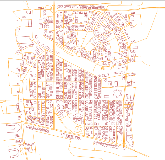
Following image shows the roads and buildings visualised.

3.2.2. Preprocessing Buildings ¶

The table buildings_ways contains the buildings in edge form. They have to be converted into polygons to get the area.

3.2.2.1. Exercise 6: Add a spatial column to the table ¶

Add a spatial column named poly_geom to the table buildings_ways to store the Polygon Geometry

SELECT AddGeometryColumn('buildings','buildings_ways','poly_geom',4326,'POLYGON',2);

Exercise: 6 (Chapter: SDG 3)

3.2.2.2. Exercise 7: Removing the polygons with less than 4 points ¶

ST_NumPoints is used to find the number of points on a geometry. Also, polygons with less than 3 points/vertices are not considered valid polygons in PostgreSQL. Hence, the buildings having less than 3 vertices need to be cleaned up. Follow the steps given below to complete this task.

DELETE FROM buildings_ways 
WHERE ST_NumPoints(the_geom) < 4 
OR ST_IsClosed(the_geom) = FALSE;

Exercise: 7 (Chapter: SDG 3)

3.2.2.3. Exercise 8: Creating the polygons ¶

ST_MakePolygons is used to make the polygons. This step stores the geom of polygons in the poly_geom column which was created earlier.

UPDATE buildings_ways 
SET poly_geom = ST_MakePolygon(the_geom);

Exercise: 8 (Chapter: SDG 3)

3.2.2.4. Exercise 9: Calculating the area ¶

After getting the polygon geometry, next step is to find the area of the polygons. Follow the steps given below to complete this task.

Adding a column for storing the area

ALTER TABLE buildings_ways
ADD COLUMN area INTEGER;

Storing the area in the new column

ST_Area is used to calculate area of polygons. Area is stored in the new column

UPDATE buildings_ways 
SET area = ST_Area(poly_geom::geography)::INTEGER;
-- Process to discard disconnected roads

Exercise: 9 (Chapter: SDG 3)

3.2.3. pgr_connectedComponents ¶

For the next step pgr_connectedComponents will be used. It is used to find the connected components of an undirected graph using a Depth First Search-based approach.

Signatures

pgr_connectedComponents(edges_sql)

RETURNS SET OF (seq, component, node)
OR EMPTY SET

pgr_connectedComponents Documentation can be found at this link for more information.

3.2.4. Preprocessing Roads ¶

pgRouting algorithms are only useful when the road network belongs to a single graph (or all the roads are connected to each other). Hence, the disconnected roads have to be removed from their network to get appropriate results. This image gives an example of the disconnected edges.

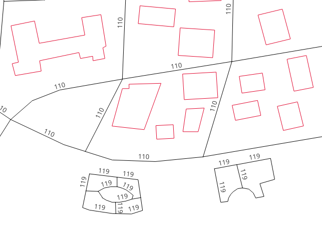
../_images/remove_disconnected_roads.png

For example, in the above figure roads with label 119 are disconnected from the network. Hence they will have same connected component number. But the count of this number will be less count of fully connected network. All the edges with the component number with count less than maximum count will be removed

Follow the steps given below to complete this task.

3.2.4.1. Exercise 10: Find the Component ID for Road vertices ¶

First step in Preprocessing Roads is to find the connected component ID for Road vertices. Follow the steps given below to complete this task.

Add a column named component to store component number.

ALTER TABLE roads_ways_vertices_pgr
ADD COLUMN component INTEGER;

Update the component column in roads_ways_vertices_pgr with the component number

UPDATE roads_ways_vertices_pgr 
SET component = subquery.component 
FROM (
	SELECT * FROM pgr_connectedComponents(
		'SELECT gid AS id, source, target, cost, reverse_cost 
		FROM roads_ways'
			)
		) 
AS subquery
WHERE id = node;

This will store the component number of each edge in the table. Now, the completely connected network of roads should have the maximum count in the component table.

SELECT component, count(*) FROM road_ways_vertices_pgr GROUP BY  component;

Exercise: 10 (Chapter: SDG 3)

3.2.4.2. Exercise 11: Finding the components which are to be removed ¶

This query selects all the components which are not equal to the component number with maximum count using a subquery which groups the rows in roads_ways_vertices_pgr by the component.

WITH
subquery AS (
	SELECT component, COUNT(*) 
	FROM roads_ways_vertices_pgr 
	GROUP BY component
	)
SELECT component FROM subquery 
WHERE COUNT != (SELECT max(COUNT) FROM subquery);

Exercise: 11 (Chapter: SDG 3)

3.2.4.3. Exercise 12: Finding the road vertices of these components ¶

Find the road vertices of these components which belong to those components which are to be removed. The following query selects all the road vertices which have the component number from Exercise 11.

WITH
subquery AS (
	SELECT component, COUNT(*) 
	FROM roads_ways_vertices_pgr 
	GROUP BY component
	),
to_remove AS (
	SELECT component FROM subquery 
	WHERE COUNT != (SELECT max(COUNT) FROM subquery)
	)
SELECT id FROM roads_ways_vertices_pgr 
WHERE component IN (SELECT * FROM to_remove);

Exercise: 12 (Chapter: SDG 3)

3.2.4.4. Exercise 13: Removing the unwanted edges and vertices ¶

Removing the unwanted edges

In roads_ways table (edge table) source and target have the id of the vertices from where the edge starts and ends. To delete all the disconnected edges the following query takes the output from the query of Step 4 and deletes all the edges having the same source as the id.

DELETE FROM roads_ways WHERE source IN (
	WITH
	subquery AS (
		SELECT component, COUNT(*) 
		FROM roads_ways_vertices_pgr 
		GROUP BY component
		),
	to_remove AS (
		SELECT component FROM subquery 
		WHERE COUNT != (SELECT max(COUNT) FROM subquery)
		)
	SELECT id FROM roads_ways_vertices_pgr 
	WHERE component IN (SELECT * FROM to_remove)
);

Removing unused vertices

The following query uses the output of Step 4 to remove the vertices of the disconnected edges.

WITH
subquery AS (
	SELECT component, COUNT(*) 
	FROM roads_ways_vertices_pgr 
	GROUP BY component
	),
to_remove AS (
	SELECT component FROM subquery 
	WHERE COUNT != (SELECT max(COUNT) FROM subquery)
	)
DELETE FROM roads_ways_vertices_pgr 
WHERE component IN (SELECT * FROM to_remove);

Exercise: 13 (Chapter: SDG 3)

3.3. Finding the roads served by the hospitals ¶

After pre-processing the data, next step is to find the area served by the hospital. This area can be computed from the entrance of the hospital or from any point on road near the hospital. In this exercise it is computed from closest road vertex. pgr_drivingDistance will be used to find the roads served. The steps to be followed are:

Finding the closest road vertex
Finding the roads served
Generalising the roads served

3.3.1. Exercise 14: Finding the closest road vertex ¶

There are multiple road vertices near the hospital. Create a function to find the geographically closest road vertex. closest_vertex function takes geometry of other table as input and gives the gid of the closest vertex as output by comparing geom of both the tables.

The following query creates a function to find the closest road vertex.

CREATE OR REPLACE FUNCTION closest_vertex(geom GEOMETRY)
RETURNS BIGINT AS
$BODY$
SELECT id FROM roads_ways_vertices_pgr ORDER BY geom <-> the_geom LIMIT 1;
$BODY$
LANGUAGE SQL;

3.3.2. pgr_drivingDistance ¶

For the next step pgr_drivingDistance will be used. This returns the driving distance from a start node. It uses the Dijkstra algorithm to extract all the nodes that have costs less than or equal to the value distance. The edges that are extracted conform to the corresponding spanning tree.

Signatures

pgr_drivingDistance(edges_sql, start_vid,  distance [, directed])
pgr_drivingDistance(edges_sql, start_vids, distance [, directed] [, equicost])
RETURNS SET OF (seq, [start_vid,] node, edge, cost, agg_cost)

Using defaults

pgr_drivingDistance(edges_sql, start_vid, distance)
RETURNS SET OF (seq, node, edge, cost, agg_cost)

Single Vertex

pgr_drivingDistance(edges_sql, start_vid, distance [, directed])
RETURNS SET OF (seq, node, edge, cost, agg_cost)

Multiple Vertices

pgr_drivingDistance(edges_sql, start_vids, distance, [, directed] [, equicost])
RETURNS SET OF (seq, start_vid, node, edge, cost, agg_cost)

pgr_drivingDistance Documentation can be found at this link for more information.

3.3.3. Exercise 15: Finding the served roads using pgr_drivingDistance ¶

In this exercise, the roads served based on travel-time are calculated. This can be calculated using pgrdrivingDistance function of pgRouting. Time in minutes is considered as cost. The agg_cost column would show the total time required to reach the hospital.

For the following query,

In line 3, Pedestrian speed is assumed to be as 1 m/s. As time = distance/speed, length_m / 1 m/s / 60 gives the time in minutes
In line 7, tag_id = '318' as 318 is the tag_id of hospital in the configuration file of buildings. Reference for Tag ID : Appendix
In line 8, 10 is written for 10 minutes which is a threshold for agg_cost
In line 8, FALSE is written as the query is for undirected graph

SELECT gid,source,target,agg_cost,r.the_geom
FROM pgr_drivingDistance(
        'SELECT gid as id,source,target, length_m/60 AS cost,length_m/60 AS reverse_cost 
        FROM roads.roads_ways',
        (SELECT closest_vertex(poly_geom) 
        FROM buildings.buildings_ways 
        WHERE tag_id = '318'
        ), 10, FALSE
      ), roads.roads_ways AS r
WHERE edge = r.gid 
LIMIT 10;

Note

LIMIT 10 displays the first 10 rows of the output.

Exercise: 15 (Chapter: SDG 3)

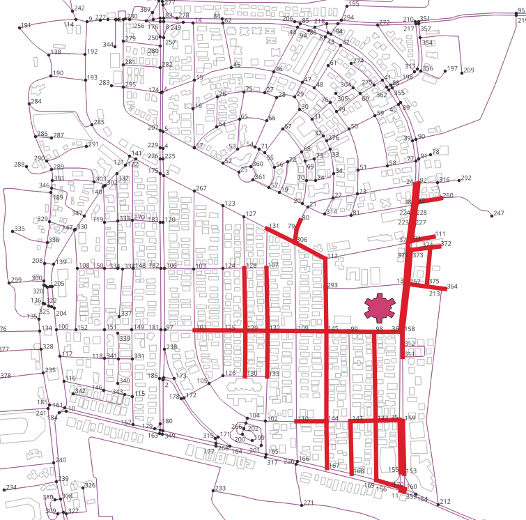
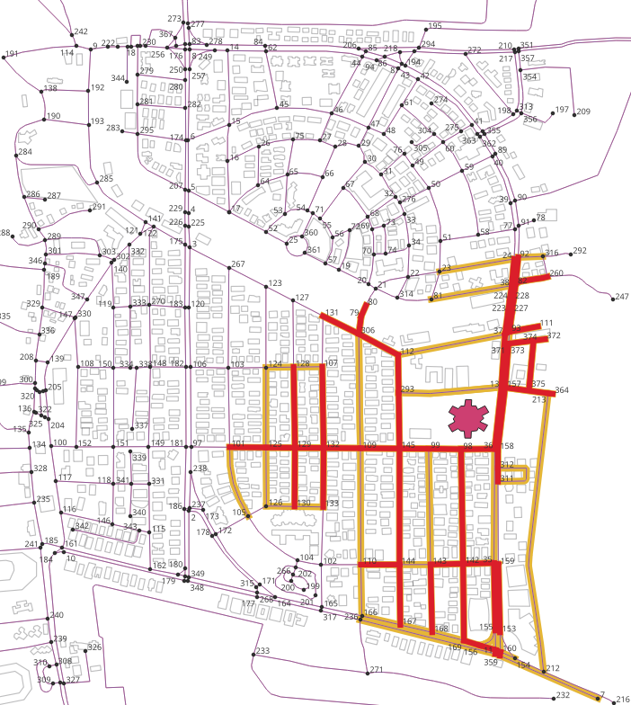
Following figure shows the visualised output of the above query. The lines highlighted by red colour show the area from where the hospital can be reached within 10 minutes of walking at the speed of 1 m/s. It is evident from the output figure that some of the roads which are near to the hospital are not highlighted. For example, to roads in the north of the hospital. This is because the only one edge per road vertex was selected by the query. Next section will solve this issue by doing a small modification in the query.

3.3.4. Exercise 16: Generalising the served roads ¶

The edges which are near to to hospital should also be selected in the roads served as the hospital also serves those buildings. The following query takes the query from previous section as a subquery and selects all the edges from roads_ways that have the same source and target to that of subquery (Line 14).

WITH subquery AS (
SELECT r.gid, edge,source,target,agg_cost,r.the_geom 
FROM pgr_drivingDistance(
        'SELECT gid as id,source,target, length_m/60 AS cost, length_m/60 AS reverse_cost 
        FROM roads.roads_ways',
        (SELECT closest_vertex(poly_geom) 
        FROM buildings.buildings_ways 
        WHERE tag_id = '318'
        ), 10, FALSE
      ),roads.roads_ways AS r
WHERE edge = r.gid)
SELECT r.gid, s.source, s.target, s.agg_cost,r.the_geom 
FROM subquery AS s, roads.roads_ways AS r 
WHERE r.source = s.source OR r.target = s.target
ORDER BY r.gid
LIMIT 10;

Note

LIMIT 10 displays the first 10 rows of the output.

Exercise: 16 (Chapter: SDG 3)

Following figure shows the visualised output of the above query. Lines highlighted in yellow show the generalised the roads served. This gives a better estimate of the areas from where the hospital can be reached by a particular speed.

3.4. Calculating the total population served by the hospital ¶

Now the next step is to estimate the dependant population. Official source of population is Census conducted by the government. But for this exercise, population will be estimated from the area as well as the category of the building. This area will be stored in the nearest roads. Following steps explain this process in detail.

3.4.1. Exercise 17: Estimating the population of buildings ¶

Population of an building can be estimated by its area and its category. Buildings of OpenStreetMap data are classified into various categories. For this exercise, the buildings are classified into the following classes:

Negligible: People do not live in these places. But the default is 1 because of homeless people.
Very Sparse: People do not live in these places. But the default is 2 because there may be people guarding the place.
Sparse: Buildings with low population density. Also, considering the universities and college because the students live there.
Moderate: A family unit housing kind of location.
Dense: A medium sized residential building.
Very Dense: A large sized residential building.

Reference: Appendix

This class-specific factor is multiplied with the area of each building to get the population. Follow the steps given below to complete this task.

Create a function to find population using class-specific factor and area.

CREATE OR REPLACE FUNCTION  population(tag_id INTEGER,area INTEGER)
RETURNS INTEGER AS 
$BODY$
DECLARE 
population INTEGER;
BEGIN 
  IF tag_id <= 100 THEN population = 1; -- Negligible
  ELSIF 100 < tag_id AND tag_id <= 200 THEN  population = GREATEST(2, area * 0.0002); -- Very Sparse
  ELSIF 200 < tag_id AND tag_id <= 300 THEN  population = GREATEST(3, area * 0.002); -- Sparse
  ELSIF 300 < tag_id AND tag_id <= 400 THEN population = GREATEST(5,  area * 0.05); -- Moderate
  ELSIF 400 < tag_id AND tag_id <= 500  THEN population = GREATEST(7, area * 0.7); -- Dense
  ELSIF tag_id > 500  THEN population = GREATEST(10,area * 1); -- Very Dense
  ELSE population = 1;
  END IF;
  RETURN population;
END;
$BODY$
LANGUAGE plpgsql;

Note

All these are estimations based on this particular area. More complicated functions can be done that consider height of the apartments but the design of a function is going to depend on the availability of the data. For example, using census data can achieve more accurate estimation.

Add a column for storing the population in the buildings_ways

ALTER TABLE buildings_ways
ADD COLUMN population INTEGER;

3. Use the population function to store the population in the new column created in the building_ways.

UPDATE buildings_ways 
SET population = population(tag_id,area)::INTEGER;

Exercise: 17 (Chapter: SDG 3)

3.4.2. Exercise 18: Finding the nearest roads to store the population ¶

To store the population of buildings in the roads, nearest road to a building is to be found. Follow the steps given below to complete this task.

Create Function for finding the closest edge.

CREATE OR REPLACE FUNCTION closest_edge(geom GEOMETRY)
RETURNS BIGINT AS
$BODY$
SELECT gid FROM roads_ways ORDER BY geom <-> the_geom LIMIT 1;
$BODY$
LANGUAGE SQL;

Add a column in buildings_ways for storing the id of closest edge

ALTER TABLE buildings_ways
ADD COLUMN edge_id INTEGER;

Store the edge id of the closest edge in the new column of buildings_ways

UPDATE buildings_ways SET edge_id = closest_edge(poly_geom);

Exercise: 18 (Chapter: SDG 3)

3.4.3. Exercise 19: Storing the population in the roads ¶

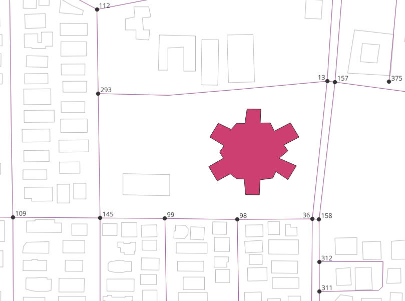
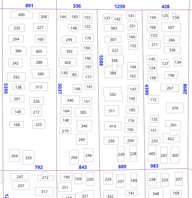
After finding the nearest road, the sum of population of all the nearest buildings is stored in the population column of the roads table. Following image shows the visualised output where the blue colour labels shows the population stored in roads.

Follow the steps given below to complete this task.

Add a column in roads_ways for storing population

ALTER TABLE roads_ways
ADD COLUMN population INTEGER;

Update the roads with the sum of population of buildings closest to it

UPDATE roads_ways SET population = SUM
FROM (
	SELECT edge_id, SUM(population) 
	FROM buildings_ways GROUP BY edge_id
	) 
AS subquery 
WHERE gid = edge_id;                                                                                                                       

Verify is the population is stored using the following query.

SELECT population FROM roads_ways WHERE gid = 441;

Exercise: 19 (Chapter: SDG 3)

3.4.4. Exercise 20: Finding total population ¶

Final step is to find the total population served by the hospital based on travel-time. Use the query from Exercise 16: Generalising the served roads as a subquery to get all the edges in the roads served. Note that s.population is added in line 14 which gives the population. After getting the population for each edge/road, use sum() to get the total population which is dependant on the hospital.

WITH subquery
AS (
	WITH subquery AS (
	SELECT r.gid,source,target,agg_cost, r.population,r.the_geom 
	FROM pgr_drivingDistance(
		    'SELECT gid as id,source,target, length_m/60 AS cost, length_m/60 AS reverse_cost 
		    FROM roads.roads_ways',
		    (SELECT closest_vertex(poly_geom) 
		    FROM buildings.buildings_ways 
		    WHERE tag_id = '318'
		    ), 10, FALSE
		  ),roads.roads_ways AS r
	WHERE edge = r.gid)
	SELECT r.gid, r.the_geom, s.population
	FROM subquery AS s,roads.roads_ways AS r 
	WHERE r.source = s.source OR r.target = s.target
	)
SELECT SUM(population) FROM subquery;

Exercise: 20 (Chapter: SDG 3)